Rheological material data

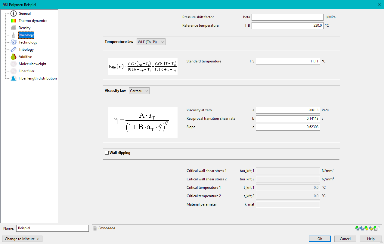
The rheological data of the material is entered in the ‘Rheology’ tab:

• Pressure shift factor beta, this input is optional. Without an input value, the pressure dependence of the viscosity is neglected.
• Reference temperature T_B, the values entered in the viscosity law are valid for this temperature.
• Temperature law, the temperature dependence of the viscosity can be modelled here. The temperature shift is calculated using PAM. The following modelling options are available
  • WLF (Tb, Ts): Temperature shift by specifying the standard temperature T_S
  • WLF (C1, C2): Temperature shift due to the constants C1 and C2
  • Arrhenius: Temperature shift due to activation energy E
• Viscosity law, the equation for describing the viscosity can be selected here. The following models are available:
  • Carreau: Input of the 3 parameters a, b and c
  • Power law: Input of the parameters K and n
• Wall slipping: If the checkbox is selected, the critical shear stress at 2 temperatures must be entered. See calculation of wall sliding

Fluids can be divided into two groups on the basis of their flow characteristics:

• Newtonian fluids
• Non-Newtonian fluids

For Newtonian fluids the following law applies:

\[τ=η\cdot\dotγ\]

with shear stress $τ$, the viscosity $η$ and the shear rate $\dotγ$.

This law states that there is proportionality between the shear stress and the shear rate, whereby the proportionality factor is the viscosity. This flow behaviour only occurs in polymer liquids or melts at very low shear rates and possibly at very high ones. Deviations are expressed in the so-called pseudoplasticity (shear thinning), dilatancy or the presence of a yield point.

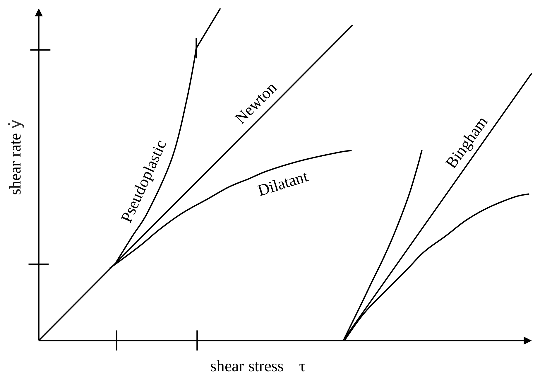
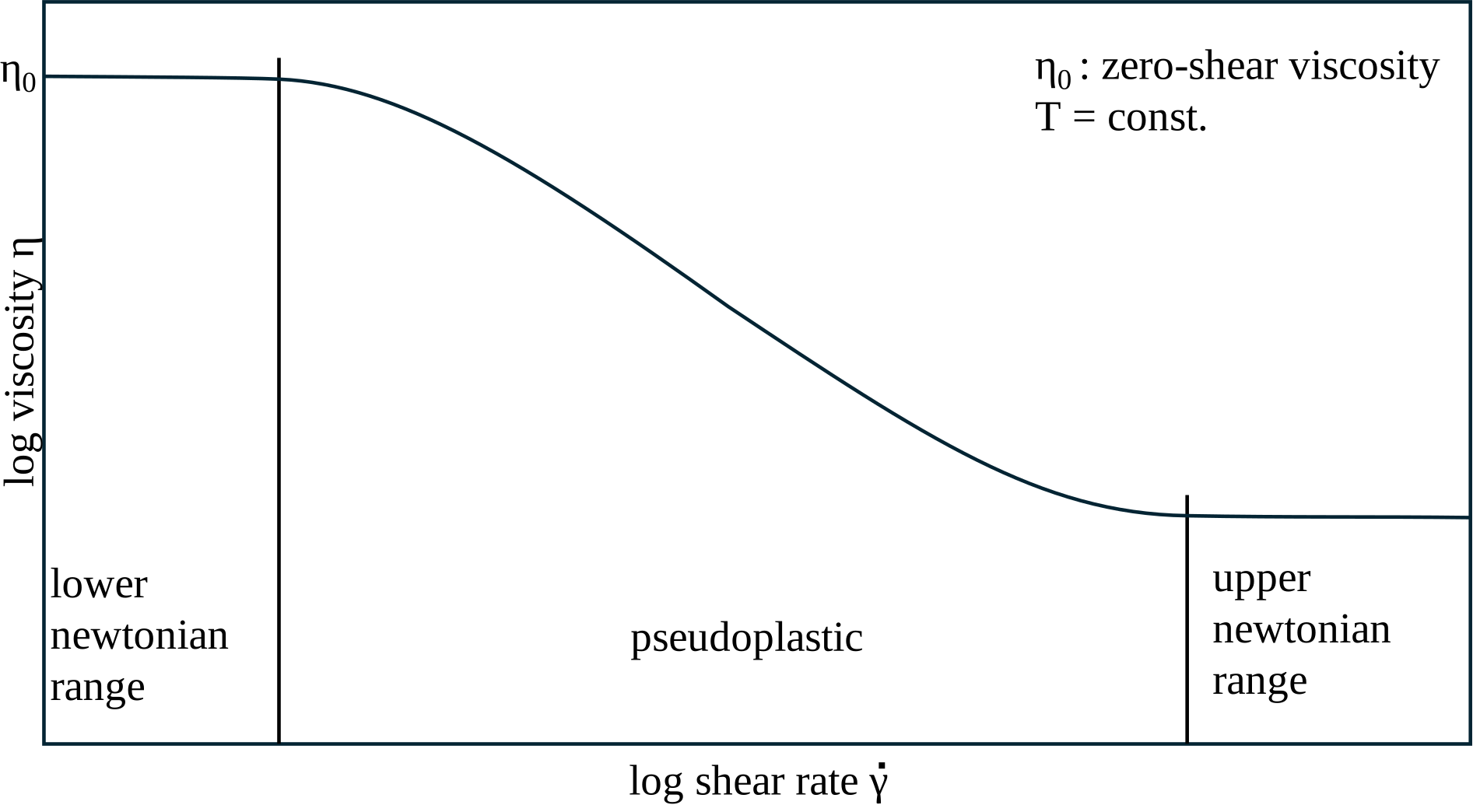
The flow behavior of polymer melts in practically relevant shear rate ranges is characterized by so-called pseudoplasticity (shear thinning). This describes a deviation from Newtonian fluid behavior, where the viscosity is no longer constant but decreases with increasing shear rate.

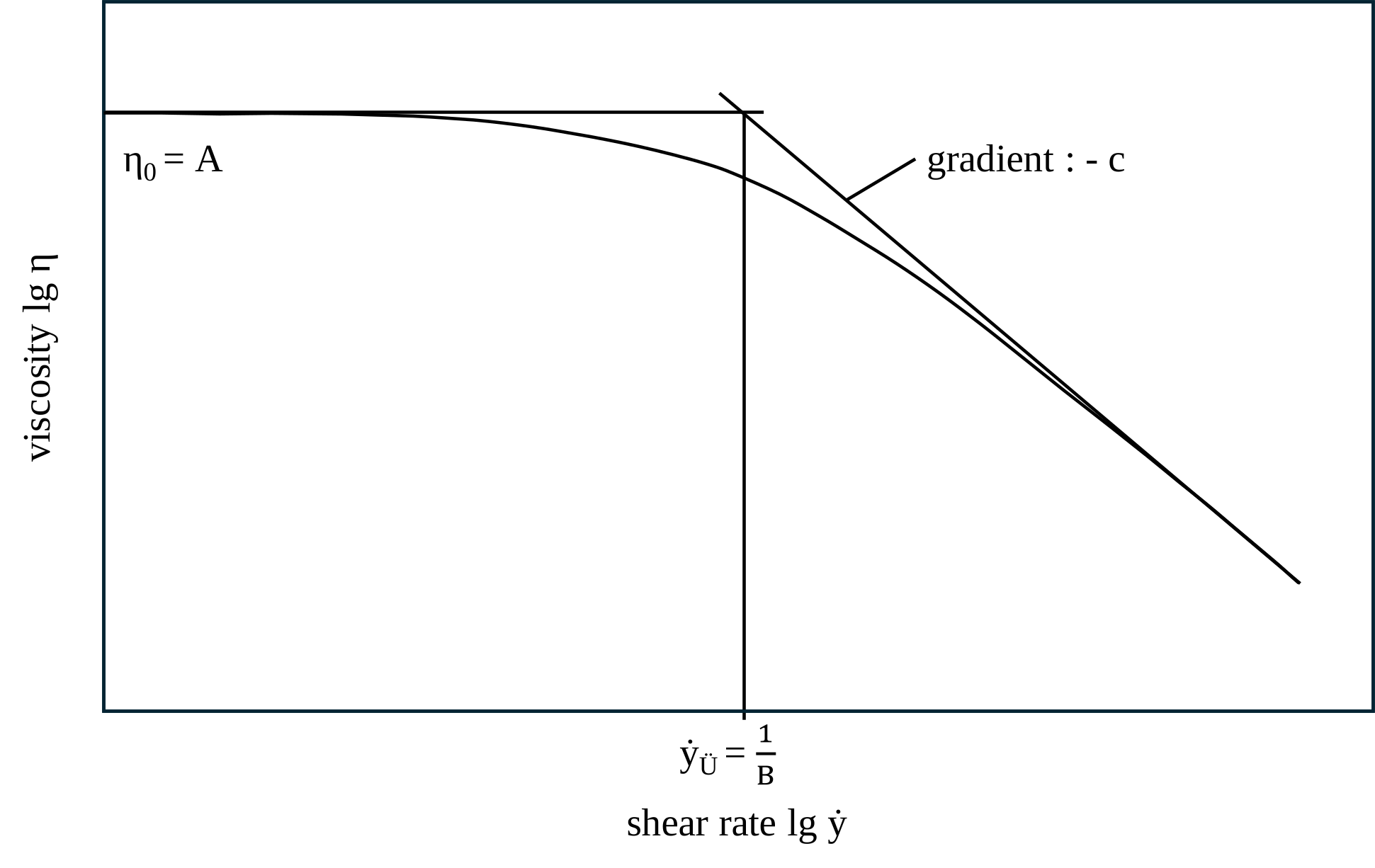
The following figure shows the basic viscosity curve as a function of the shear rate.

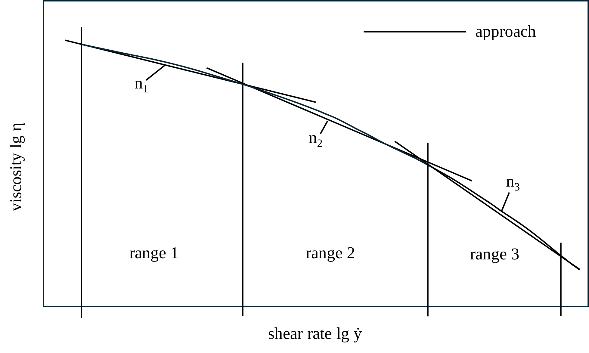
For shear rate ranges that are not too large, this behaviour can be described by the empirically found power flow law according to OSTWALD and DE WAELE:

$$τ=K\cdot\dotγ^n$$ respectively $$\eta=a_T \cdot K \cdot \gamma^{n-1}$$

where $n$ is the exponent of the flow law and $K$ is the consistency factor.

Due to the simple structure of this approach, almost all flow problems can be treated analytically. In double logarithmic representation, a straight line results for the power law. For the Newtonian range, this results in $n=1$ and $K=\eta_0$. In the pseudoplastic range, the viscosity curve in small ranges can also be approximated by the power law. This results in a shear rate-dependent $n<1$.

The CARREAU approach offers a better description over wide ranges of the viscosity function, especially for materials with a pronounced transition from the Newtonian to the pseudoplastic range:

\[η = \frac {A \cdot a_T} {(1+a_T \cdot B \cdot \dotγ)^C}\]

Where $A$ is the zero-shear viscosity, $B$ is the reciprocal transition shear rate and $C (= 1-n)$ is the gradient.

The temperature dependence is taken into account by the temperature shift factor $a_T$, which can be described in three different ways

\[log(a_T) = \frac {C_1\cdot(T_B-T_S)} {C_2+(T_B-T_S)} - \frac {C_1\cdot(T-T_S)} {C_2+(T-T_S)}\]

$T_B$, $T_S$ must be provided, $C_1 = 8,86$, $C_2 = 101,6$

with: $T_B$ = reference temperature, $T_S$ = standard temperature, $T$ = current temperature

\[ln(a_T) = - \frac {C_1 \cdot (T-T_B)} {C_2+(T-T_B)}\]

$C_1$, $C_2$, $T_B$ must be provided

with: $T_B$ = reference temperature, $T$ = current temperature

$$ln(a_T)=\frac{E}{R} (\frac{1}{T}-\frac{1}{T_B}) $$

with: $E$ = activating energy, $R$ = gas constant, $T_B$ = reference temperature (in kelvin), $T$ = current temperature (in kelvin)

The pressure shift factor beta takes into account the influence of the pressure on the viscosity. By default, the value refers to a reference pressure of 100 bar. The pressure shift $a_p$ is included in the viscosity calculation in the same way as the temperature shift factor $a_T$. $a_p$ is calculated as follows:

$$ a_p = exp(\beta \cdot (p-p_B))$$

with the pressure shift factor $\beta$, the pressure $p$ and the reference pressure $p_B$.

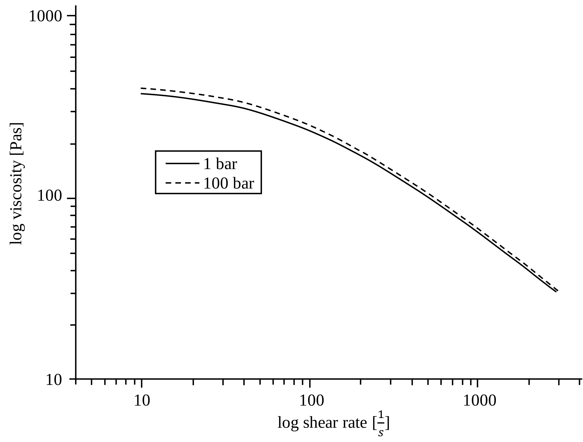
The value beta can be imported directly from PAM or entered manually. If 0 is entered as the value for beta, the viscosity is calculated without considering the pressure.

• Database connection to PAM
• General material data
• Thermodynamic data
• Density data or specific volume
• Rheological material data
• Technological data
• Tribological data
• Additives
• Molecular weight
• Fiber degradation
• Define mixture