Dies ist eine alte Version des Dokuments!
Post-Processing
After completion of a numerical REX3D simulation, various options are available for evaluating and visualizing the calculated results. Post-processing makes it possible to clearly present the simulation results and prepare them for further evaluation.
The available functions and evaluation options differ depending on the flow solver used. The following sections describe post-processing for OpenFOAM and FeatFlow.
Post-Processing (OpenFOAM)
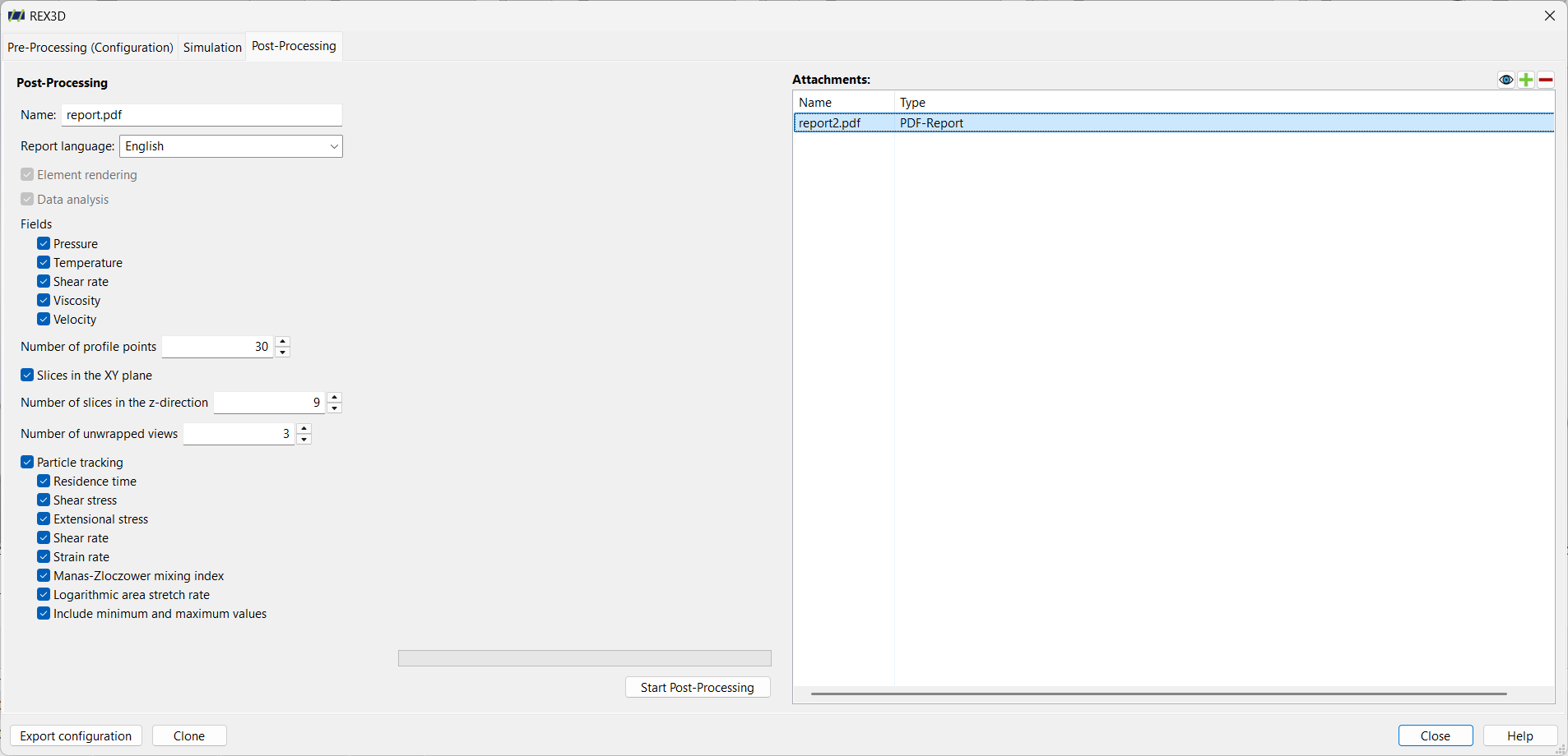
Post-Processing Settings
After a 3D simulation using OpenFOAM, automated post-processing can be performed. The result of the post-processing is always a PDF report, which can be configured and generated via the REX user interface.
Post-Processing Placeholder
Configuration Placeholder
PDF Report
The PDF report can be customized as shown above. Depending on the configuration, the corresponding pages are generated or omitted, meaning that the length of the report may vary. \ The possible pages are described below.
Cover Page

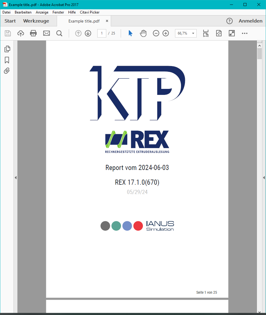
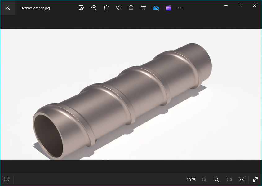
In addition to an isometric representation of the simulated screw section, the cover page contains the configuration name used in the REX/PSI user interface, the date, and the REX/PSI version used.
This allows quick traceability of when the simulation was performed and which element or elements were simulated.
Process Data

The process data overview page consists of four sections.
Graphical Representation
The element is shown here in front and side views. The green arrow below the side view indicates the conveying direction. The smaller arrow at the side indicates the direction of rotation and describes the direction of motion of the side of the element facing the viewer.
Results
The most important simulation parameters are listed here. These include:
- mass flow rate,
- pressure difference,
- temperature difference,
- mean pressure throughout the entire flow domain,
- mean temperature throughout the entire flow domain,
- mean absolute velocity throughout the entire flow domain,
- mean shear rate throughout the entire flow domain,
- mean viscosity throughout the entire flow domain, and
- mean density throughout the entire flow domain. * Listenpunkt
Process Data
Additional boundary conditions describing the operating point are listed here. These include:
- rotational speed,
- inlet temperature (at the beginning of the element),
- screw temperature (or adiabatic boundary condition), and
- barrel temperature (or adiabatic boundary condition).
Machine
The basic machine and element data are listed here. These include:
- the geometry origin (generated by REX/PSI or imported geometry),
- the name of the screw (name from REX/PSI),
- the outer diameter,
- the core diameter (smallest diameter within the simulated screw section),
- the length excluding the inlet and outlet sections, and
- the absolute length.
Material Data

This page lists the material data used in the simulation, starting with:
- the material name and
- the material type.
The thermodynamic data and density are then displayed:
- Thermal conductivity at 0°C and its slope per °C
- Heat capacity at 0°C and its slope per °C
- Melt density at 0°C and the reduction in density per °C
Finally, the Rheological Data are listed. This starts with the temperature shift, followed by the viscosity. Different parameters are listed depending on the selected model.
To visualize the viscosity, a diagram with flow curves for three different temperatures is shown. These are the inlet temperature (see Process Data), as well as temperatures 20 °C below and above the inlet temperature.
Cross-Sections and Profiles
The following pages provide a more detailed evaluation of the data. The fields „Pressure“, „Temperature“, „Shear Rate“, „Viscosity“, and „Velocity“ are evaluated one after another.
Four „evaluation methods“ are available for each field:
* Display of the profile in the axial direction with minimum, mean, and maximum values * Cross-sectional images in the Y-Z and X-Z planes * Cross-sectional images orthogonal to the axial direction at different z-coordinates * Unwrapped representations at constant radii


Particle Tracking
Particle tracking marks the beginning of a new evaluation section. Automated particle tracking is performed and evaluated in various ways. Details are described in the following sections. All results shown here are based on the simulated streamlines of massless particles.
Evaluating the streamlines, with the exception of simply examining the particle distribution for assessing distributive mixing, is memory-intensive. In many cases, more memory is required than for the flow simulation itself.
The distributive mixing performance can be evaluated using the mixing quality $MQ$ described below.
Dispersive mixing quality mainly depends on the occurring elongational and shear stresses, which are also evaluated. In addition, the Manas-Zloczower mixing index and the logarithmic area stretch can be used as supplementary criteria for evaluation.
Graphical Representation

First, a purely subjective evaluation is provided by displaying a small number of streamlines that are evenly distributed at the inlet. This representation is intended to allow a subjective assessment of the flow behavior within the simulated screw section.
Distributive Mixing

This page provides a mathematical evaluation of the distributive mixing performance. Since this evaluation depends on the flow channel cross-section, the elements are always generated with defined inlet and outlet sections in order to obtain reproducible and comparable results.
The inlet is divided so that streamlines start in two opposing eighths of the flow channel. These are calculated separately and are also evaluated separately at the outlet. The more uniform the particle distribution at the outlet, the better the distributive mixing performance.
Approximately 2000–2500 streamlines start in each eighth, although this value may vary slightly depending on the diameter. Since streamlines are calculated using discrete time steps and therefore discrete path increments, some streamlines may leave the flow domain due to discretization effects and consequently fail to reach the outlet. A loss of up to 20% is considered acceptable. Higher losses may negatively affect the reliability of the particle-tracking results.
The particle distribution at the outlet is used to evaluate the distributive mixing quality. The bounding inner and outer diameters of the cross-section are also represented by points whose statistical spacing corresponds to that of an optimal particle distribution. Based on the boundary points and the outlet points from the particle tracking, a Delaunay triangulation is performed. This creates triangles between the points according to defined criteria. These triangles consequently have individual areas. The distributive mixing quality is determined from the distribution of these areas, more specifically from the coefficient of variation $CV$ of the area distribution.
\( MQ = \frac{CV_{best}}{CV}\)
$CV_{best}$ is fixed at a value of $0.75$. This ensures that very good mixing elements can achieve a mixing quality above 0.9 while preventing a mixing quality greater than 1. The mixing quality $MQ$ is therefore a characteristic value between $0$ and $1$.
The averaged mixing quality is calculated as the arithmetic mean of the mixing qualities of the two initial distributions.
Residence Time Distribution

The residence time distribution describes the time required for the particles to flow through the element. Depending on the material and the desired mixing effect, either a narrow or a broad distribution may be preferable.
The residence time refers only to the simulated screw section WITHOUT the inlet and outlet sections.
Shear Stress
The shear stress $\tau$ is evaluated for each individual streamline. The following applies:
\( \tau = \eta \cdot \dot{\gamma}\)
with the viscosity $\eta$ and the shear rate $\dot{\gamma}$.
Each streamline therefore has its own individual shear-stress profile. The shear stress is also integrated over time, meaning that each streamline has a minimum, maximum, and time-integrated value. The time-weighted mean value is additionally calculated by dividing the integrated value by the residence time.
The sum of all streamlines therefore produces distributions for the minimum, mean, maximum, and integrated values.


Elongational Stress
The elongational stress $\sigma$ is evaluated in a similar manner to the shear stress. However, the elongational stress is calculated using:
\(\sigma = \eta_{dehn} \cdot \dot{\epsilon}\)
with the elongational viscosity according to the Trouton ratio:
\(\eta_{dehn} = 3 \cdot \eta\)
The calculation of the elongation rate $\dot{\epsilon}$ is described below.


Shear Rate
The shear rate $\dot{\gamma}$ is calculated using:
\(\dot{\gamma} = \sqrt{2 D:D}\)
The minimum, mean, maximum, and time-integrated shear rates are evaluated for each streamline. The sum of the streamlines produces a corresponding distribution for each value.


Elongation Rate
The elongation rate $\dot{\epsilon}$ is the maximum positive principal strain rate of the deformation tensor $D$, which is calculated from the velocity gradient $\nabla u$.
\( \dot{\epsilon} = max(0,\lambda_{max}(D))\)
\( D = \frac{1}{2} (\nabla u + (\nabla u)^T)\)
The deformation tensor $D$ has the three eigenvalues $\lambda_1$, $\lambda_2$, and $\lambda_3$.


Manas-Zloczower Mixing Index

The Manas-Zloczower mixing index is calculated from the vorticity tensor $W$ and the deformation tensor $D$:
\( Mixing\ Index = \frac{|D|}{|D|+|W|}\)
\( W = \frac{1}{2} (\nabla u - (\nabla u)^T)\)
\( D = \frac{1}{2} (\nabla u + (\nabla u)^T)\)
The deformation tensor is a measure of how strongly a fluid element is deformed. The vorticity tensor is a measure of the rotational motion of the flow.
The following limiting cases can occur:
* $|D|=0$ \ $Mixing\ Index = 0.0$ \ This represents pure rotational flow. * $|D|=|W|$ \ $Mixing\ Index = 0.5$ \ This represents pure shear flow. * $|W|=0$ \ $Mixing\ Index = 1.0$ \ This represents pure elongational flow.
Since this is only a local quantity, neither minimum nor maximum values are specified. Only the residence-time-weighted mean mixing index is shown.
Logarithmic Area Stretch
The logarithmic area stretch ln($\lambda$) is a measure of how strongly an area is stretched by the local velocity gradients. The higher the value, the greater the area stretching experienced by an infinitesimally small area along the streamlines. The value depends on the occurring elongation rates and is a measure of elongational flow and therefore also of dispersive mixing.
The following applies:
\(\lambda = \frac{A}{A_0}\)
The local logarithmic rate of change of the stretch is calculated using:
\( \frac{d}{dt}ln(\lambda) = \text{div}(u) - n^T \cdot D \cdot n\)
The divergence of the velocity field div(u) is equal to 0 for incompressible media. \ The deformation tensor $D$ has already been explained above. \ $n$ is the unit normal vector of the area under consideration, which also changes as a result of the flow.
Since the normal vector is included in the calculation, the orientation of the initial area influences the calculated result. For each streamline, the initial orientation is rotated through normal vectors in the x-, y-, and z-directions. A mean value is then calculated from these orientations.
Integration over time yields $ln(\lambda)$, the logarithmic area stretch described in the first paragraph.


Post-Processing (FeatFlow)
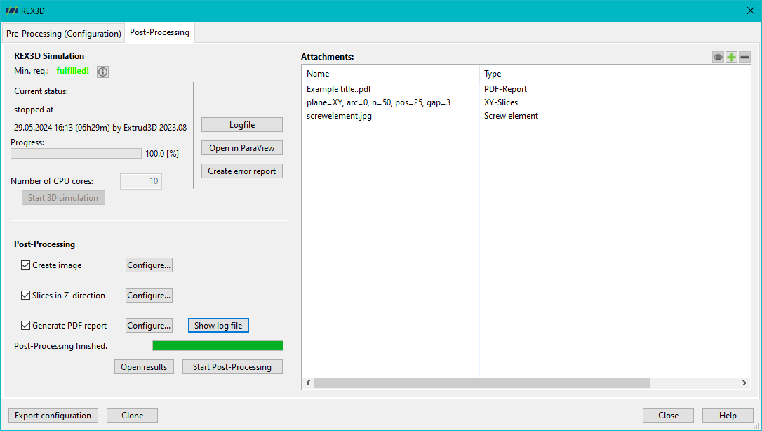
After a simulation has been successfully completed, various post-processing steps can be performed:\
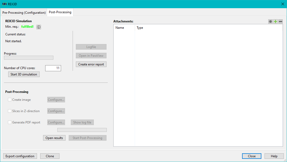
Various configuration options are available for the individual post-processing steps:\
Generate Image File
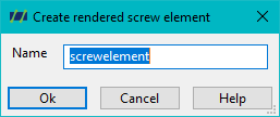
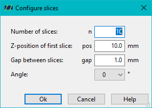
Cross-Sections in Z-Direction
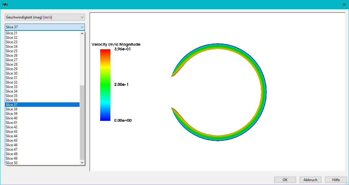
For cross-sections in the Z-direction, it is possible to select the number of cross-sections, the Z-position of the first cross-section, and the distance between the cross-sections. If several time levels have been simulated, the time level or screw position to be evaluated can be selected using the angle. If only one time level has been simulated, only one angular position is available accordingly.\
Generate PDF Report
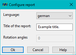
Post-processing also provides the option of generating a PDF report containing a general evaluation of the flow simulation. Before the PDF report is generated, the language and title of the report can be defined.
Once the various post-processing functions have been performed, their results can be accessed in the Attachments field. An example is shown in the following figure, which displays the flow velocity on an XY cross-sectional plane.\
Display Results in the Attachments
The storage location of the files that have already been generated can be accessed using the Display results of a numerical 3D simulation button or via the navigation path: Simulation > Open REX3D Diagram. \
PDF Report
The PDF report provides a clear summary of the numerical results.
Cross-Sections in Z-Direction
Rendered Screw Element