Dies ist eine alte Version des Dokuments!
ScaleUp module
If a process is to be scaled to a new machine size, this is possible with the Scale-Up module. The module is called up via Process > Scale-Up.
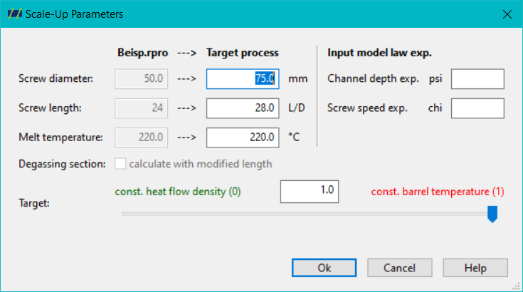
Operation of the scale-up module
The Scale-Up module offers the option of scaling processes to larger or smaller production plants. It enables the adjustment of critical process variables and the simulation of the effects of these changes. The module is operated via the menu item Project Scale-Up, which takes you to a detailed dialogue window in which both output variables of the current process and adjustments for the target process can be made.
Output variables of the process
The dialogue box that opens first displays the output variables of the process that describe the current operation of the machine. These variables include:
- Screw diameter: The diameter of the screw, which influences the conveying capacity and the pressure build-up in the extruder.
- Screw length: The length of the screw, which is decisive for material preparation and pressure build-up.
- Mass temperature: The temperature of the melted plastic material, which influences the material properties and flow characteristics.
These parameters define the starting point for the calculation and simulation of a scaled process.
Determining the target variables
You can define new variables for the target process that correspond to the requirements of the new machine or the new process. This provides flexibility to adapt the process to different machines or requirements. If the target process contains a degassing zone, the Scale-Up module offers the option of calculating a modified length of the screw including the degassing zone. This is particularly important in order to correctly map the material flow and pressure conditions in the extruder.
Creating and simulating the scaled process
By pressing the OK button, the scaled process is created and simulated based on the adjustments made. The simulation provides a detailed calculation that allows you to understand the effects of the changes on the process.
Calculation report and analysis
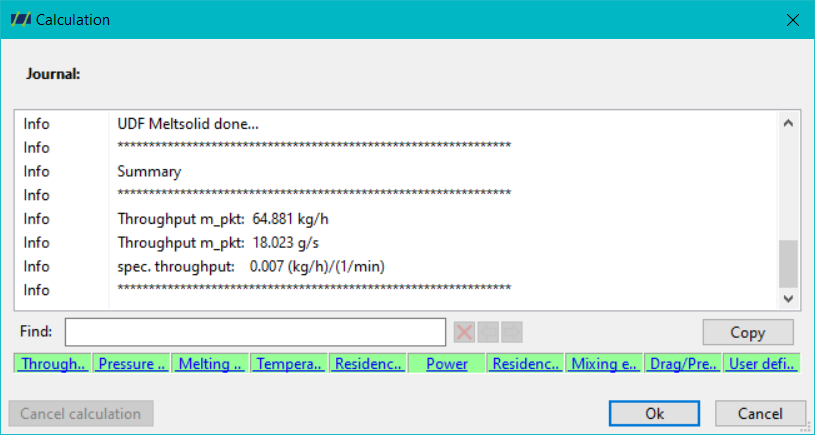
After the calculation, a calculation log opens, which shows the results of both processes - the initial process and the target process - in detail. This makes it easy to compare and check the calculations.
Pressing the OK button again opens the analysis window, in which the diagram of the model law exponents is displayed in the first step. In this diagram, the speed exponent (Psi) is shown on the X-axis. The gear depth exponent (Chi) is shown on the Y-axis.
This graphical representation allows you to analyse the interactions between speed and gear depth and to understand their influence on the process. You also have the option of analysing and comparing the results of the two processes, i.e. the initial process and the target process, in detail. Below the diagrams, you can show and hide the two machines involved in the scale-up process. This enables a direct visual comparison of the process parameters and machine configurations.
Creation of the scaled process
If the scaled process meets the desired requirements, you can create it by clicking the Create process button. This takes the simulated process as the new starting point for the actual production.
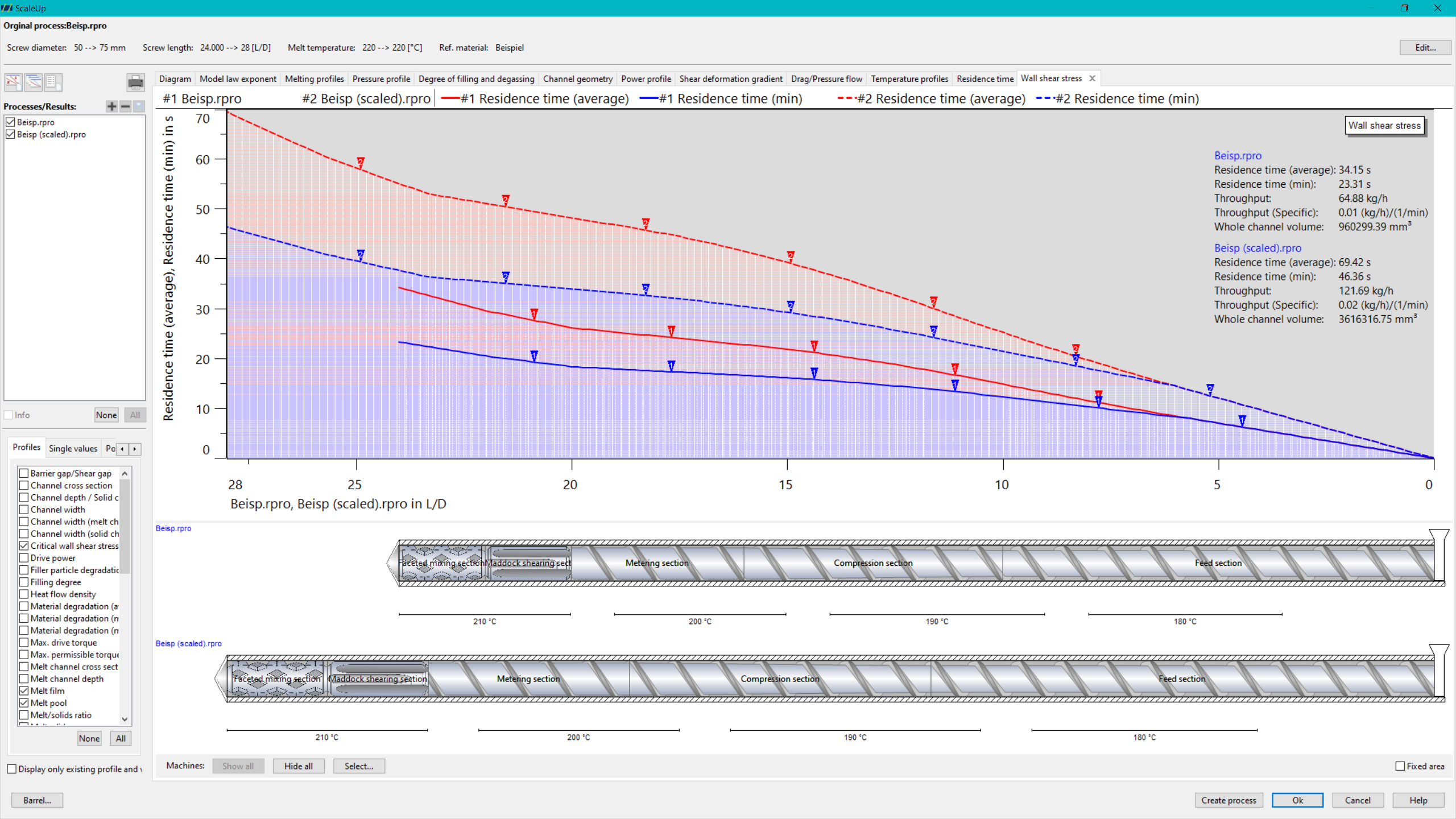
The aim of the scale-up is to generate a process with a larger or smaller diameter while maintaining or changing the screw length and maintaining or changing the final melt temperature. The screw diameter or the screw length must be changed in comparison to the initial process.
Theoretical principles
The scale-up module is based on the similarity theory based on dimensionless key figures. The dimensionless key figures should be identical for the initial process and for the scaled process so that similar process behaviour can be achieved.
The scale-up exponents $\chi$ (Chi) and $\Psi$ (Psi) are calculated from the parameters entered. Alternatively, these can also be entered manually in the input mask.
The naming of the underlying exponents is explained in the following table:
| Name | Formula symbol | Meaning | Equation |
|---|---|---|---|
| Epsilon | $\epsilon$ | pitch exponent (always 1 in REX) | $\epsilon = log\left( \frac{tan(\varphi)}{tan(\varphi_0)}\right) \bigg/ log\left( \frac{D}{D_0}\right) +1$ |
| kappa | $\kappa$ | viscosity shear rate exponent | $\kappa = -log\left( \frac{\eta}{\eta_0}\right) \bigg/ log\left( \frac{\dot{\gamma}}{\dot{\gamma}_0}\right)$ |
| Xi | $\xi$ | mass temperature exponent | $\xi = -log\left( \frac{\vartheta}{\vartheta_0}\right) \bigg/ log\left( \frac{\dot{\gamma}}{\dot{\gamma}_0}\right)$ |
| Omega | $\omega$ | length exponent | $\omega= log\left( \frac{\frac{\frac{L}{D}}{\left( \frac{L}{D}\right)_0}\right) \bigg/ log\left( \frac{D}{D_0}\right)$ |
with
| Formula symbol | Meaning |
|---|---|
| $\varphi$ | Gradient |
| $\eta$ | viscosity |
| $\dot{\gamma}$ | shear rate |
| $\vartheta$ | temperature |
| $L$ | length of the screw |
| $D$ | Nominal diameter extruder |
When calculating the scale-up exponents $\chi$ (Chi, speed exponent) and $\Psi$ (Psi, gear depth exponent), a case distinction is made. A distinction is made between
- Diameter remains the same
- Diameter does not remain the same
and
- constant cylinder temperature: Assumption in similarity theory that the temperature difference between plastic melt and cylinder temperature remains identical.
- constant heat flux density: Assumption that the area-related heat flow of the cylinder temperature control remains identical.
For the scaled process, however, the second assumption means that the cylinder temperature settings must be searched for on the system for which the surface-related heat flow is identical to that of the initial process.
However, as this is not usually the case and an identical temperature profile is used, the accuracy of the scaled process is reduced. However, higher throughputs are achieved with the assumption of constant heat flux density than with the assumption of constant cylinder temperature. A compromise can be concluded from both assumptions, so that a higher throughput is possible at the expense of scaling accuracy compared to the assumption of constant cylinder temperature.
This compromise can be set in REX using the ‘Target’ slider in the input screen. By default, the standard assumption of constant cylinder temperature is used due to the better scaling accuracy. However, the slider allows a setting at any position between the described boundary conditions.
| Case 1: Diameter unequal, constant cylinder temperature |
|---|
| $\Psi=\frac{(2+\omega-\epsilon)(2-\kappa)}{4-3\kappa+2\xi}$ |
| $\chi=\frac{\Psi(2+\xi)-(1+\omega-\epsilon+\xi)}{1-\xi}$ |
| Case 2: Diameter unequal, constant heat flux density |
|---|
| $\Psi=\frac{(2+\omega-\epsilon)(2-\kappa)}{3-2\kappa+\xi}$ |
| $\chi=\frac{\Psi(1+\xi)-(1+\omega-\epsilon+\xi)}{1-\xi}$ |
| Case 3: Diameter equal, constant cylinder temperature |
|---|
| $\Psi=\frac{2-\kappa}{4-3\kappa+2\xi}$ |
| $\chi=\frac{\Psi(2+\xi)-1}{1-\xi}$ (smooth tube extruder) |
| $\chi=\frac{\Psi(1+2\xi)-\xi}{1-\xi}$ (Nutbuchsenextruder) |
| Case 4: Diameter equal, constant heat flux density |
|---|
| $\Psi=\frac{2-\kappa}{3-2\kappa+\xi}$ |
| $\chi=\frac{\Psi(1+\xi)-1}{1-\xi}$ (smooth tube extruder) |
| $\chi=\frac{\xi(2\Psi-1)}{1-\xi}$ (grooved barrel extruder) |
The most important process and geometry parameters are calculated as follows:
| Screw length |
|---|
| $\frac{L}{L_0}=\left( \frac{D}{D_0} \right)^{1-\omega}$ |
| Gear depth |
|---|
| $\frac{h}{h_0}=\left( \frac{D}{D_0} \right)^{\Psi(1+\xi)-\chi(1-\xi)+(2-\xi)}$ (diameter unequal, smooth tube extruder) |
| $\frac{h}{h_0}=\left( \frac{D}{D_0} \right)^{(3-2\xi+2\xi\Psi)-\chi(1-\xi)+\omega(1-\xi)}$ (unequal diameter, grooved barrel extruder) |
| $\frac{h}{h_0}=\left( \frac{L}{L_0} \right)^{\Psi(1+\xi)-\chi(1-\xi)}$ (diameter equal, smooth tube extruder) |
| $\frac{h}{h_0}=\left( \frac{L}{L_0} \right)^{2\Psi\xi+(1-\xi)(1-\chi)}$ (diameter equal, grooved barrel extruder) |
| Speed |
|---|
| $\frac{n}{n_0}=\left( \frac{D}{D_0} \right)^{-\chi}$ (diameter unequal) |
| $\frac{n}{n_0}=\left( \frac{L}{L_0} \right)^{-\chi}$ (diameter equal) |
| Throughput |
|---|
| $\frac{\dot{m}}{\dot{m}_0}=\left( \frac{D}{D_0} \right)^{2+\Psi-\chi}$ (diameter unequal, smooth tube extruder) |
| $\frac{\dot{m}}{\dot{m}_0}=\left( \frac{D}{D_0} \right)^{3+\omega-\chi}$ (diameter unequal, grooved barrel extruder) |
| $\frac{\dot{m}}{\dot{m}_0}=\left( \frac{L}{L_0} \right)^{\Psi-\chi}$ (diameter equal, smooth barrel extruder) |
| $\frac{\dot{m}}{\dot{m}_0}=\left( \frac{L}{L_0} \right)^{1-\chi}$ (diameter equal, grooved barrel extruder) |
Sources
- Potente, Helmut: Auslegen von Schneckenmaschinen-Baureihen. Modellgesetze und ihre Anwendung. Kunststoff-Fortschrittsberichte, Band 6, Hanser Verlag, 1981. ISBN: 3-446-13384-4
Modified length of degassing zones
When creating the scale-up, the option calculate modified length can be selected for degassing extruders.
If this setting is selected, the length of degassing zones is not calculated using the mathematical approaches described above, but with the aim of maintaining the degassing performance.
For this purpose, the specific surface renewal $\pi_{degassing}=\frac{\dot{m}}{\dot{A}_{degassing}} \thickapprox \left( \frac{D}{D_0}\right) ^{\varphi-\omega}$ with the pitch angle $\varphi$ and the dimensionless residence time $\frac{t_v}{t_{v,0}} = \left( \frac{D}{D_0}\right) ^{\omega+\chi}$ are used. From these two dimensionless considerations, the length exponent for degassing zones is $\omega = \frac{\varphi-\chi}{2}$.
When scaling the entire screw, the lengths of the scaled degassing zones are first calculated and the remaining residual length of the screw is taken into account according to the mathematical relationships in the upper section.
Sources
- Pohl, Max: High-Speed-Extrusion amorpher Polymere am Beispiel von Polycarbonat (PC) und Polymethylmethacrylat (PMMA). Dissertation, Universität Paderborn, 2019
- Schuler, W.: Degassing during polymer production and processing. Tagungsband: Varius Aspects of Ethylene-Porpylene Based Polymers, Academia-Erasme, Louvain-La-Neuve, 1991
Creating a scaled process
After entering the machine size for the scale-up / scale-down and confirming with OK, the scaled process is created and calculated automatically. After the calculation, a new window opens in which the scale-up exponents are displayed. The Diagram tab displays the pressure and melting curve for the basic and scaled process by default. The diagram can be customised using the selection at the bottom left of the window.
Placeholder image Window after calculation
The buttons at the top left of the window can be used to create additional diagram windows, open all standard diagrams or open a tabular overview of the initial and scaled process.
If the scaled process is to be saved, this can be done using the Create process button. A new window opens to specify the file name and storage location.